
opencvで画像の2値化処理する際に使用する基本的な処理をまとめました。
jupyterlab上での実行を前提としています。
関連パッケージのインポート・設定
import cv2
import matplotlib.pyplot as plt
import seaborn as sns
import numpy as np
from ipywidgets import widgets, fixed
sns.set(font='Yu Gothic')
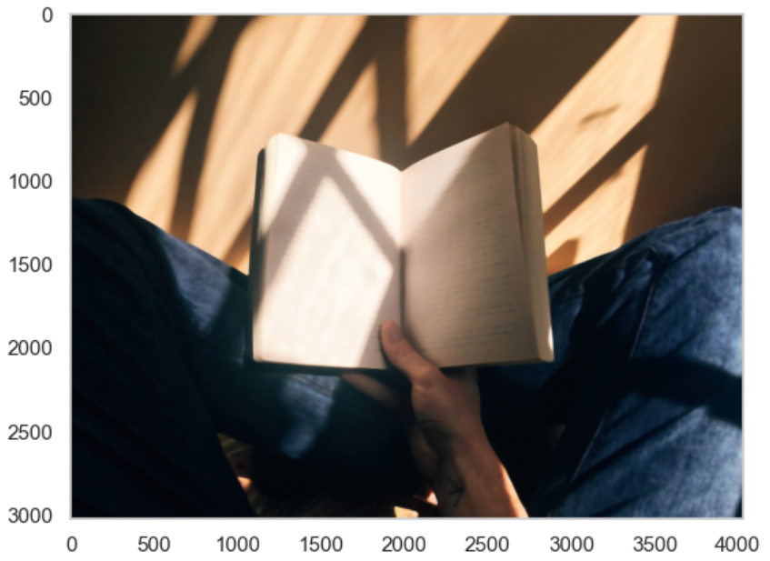
sns.set_style("whitegrid", {'axes.grid' : False})画像の読み込み
img_gray = cv2.imread('test_book.jpg',flags=cv2.IMREAD_GRAYSCALE) # グレースケール
img_color = cv2.imread('test_book.jpg',flags=cv2.IMREAD_COLOR) # カラー BGRの3チャネル RGBでない
色空間の変換
img_rgb = cv2.cvtColor(img_color, cv2.COLOR_BGR2RGB) # BGRからRGBへの変換
img_hsv = cv2.cvtColor(img_color, cv2.COLOR_BGR2HSV_FULL) # H:色相 S:彩度 V:明度
画像の表示
plt.imshow(img_gray,cmap='gray')
plt.show()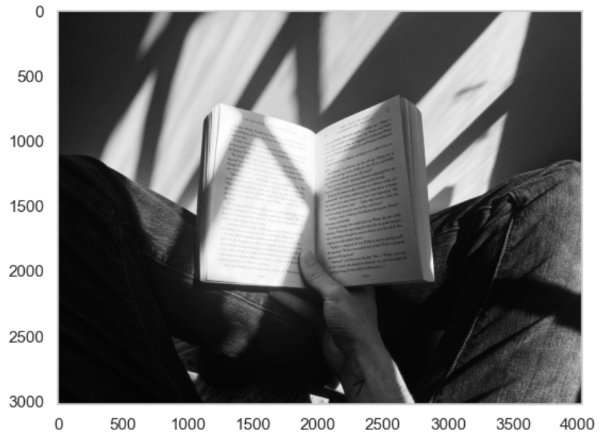
plt.imshow(cv2.cvtColor(img_color, cv2.COLOR_BGR2RGB))# チャネル順をBGRからRGBに変換する必要がある
plt.show()
チャネルごとの画像の表示
plot_img = img_rgb
color_map_list = ['Reds','Greens','Blues']
fig = plt.figure()
for i in range(len(color_map_list)):
    plt.subplot(3,1,i+1)
    plt.imshow(plot_img[:,:,i],cmap=color_map_list[i])
    plt.colorbar()
fig.set_figheight(10)
fig.set_figwidth(20)
plt.show()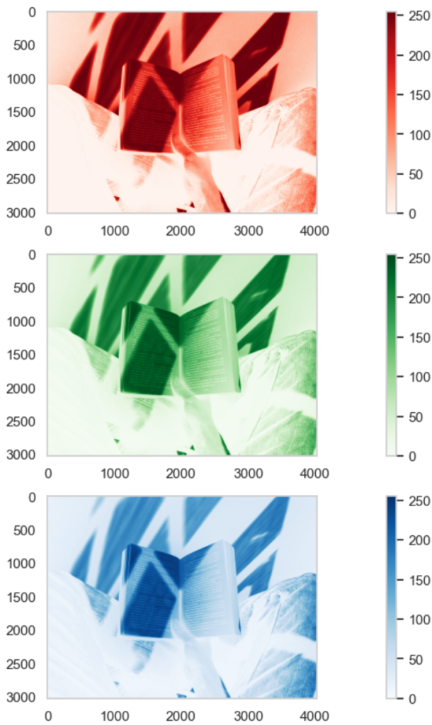
色範囲ごとの画像の表示
jupyter lab上に簡単なGUIアプリを作成します
ipywigetを活用し、指定範囲の色空間の画像を表示させます。
def create_cvrange(slide_img, chanel0, chanel1, chanel2):
    """2値化レンジを設定し、表示する"""
    lower = np.array([chanel0[0], chanel1[0], chanel2[0]])
    upper = np.array([chanel0[1], chanel1[1], chanel2[1]])

    bin_img = cv2.inRange(slide_img, lower, upper)
    plt.imshow(bin_img)

def create_slider_list(name_list):
    # スライダー設定
    param = {}
    for i, name in enumerate(name_list):
        slider =  widgets.IntRangeSlider(value=[0, 255], min=0, max=255, step=1, description=name)
        param[f'chanel{i}'] = slider
    return param

# 設定値
name_list = ["H", "S", "V"]
slide_img = img_hsv
param = create_slider_list(name_list)

# ウィジェットを表示する。
widgets.interactive(create_cvrange, slide_img=fixed(slide_img),**param)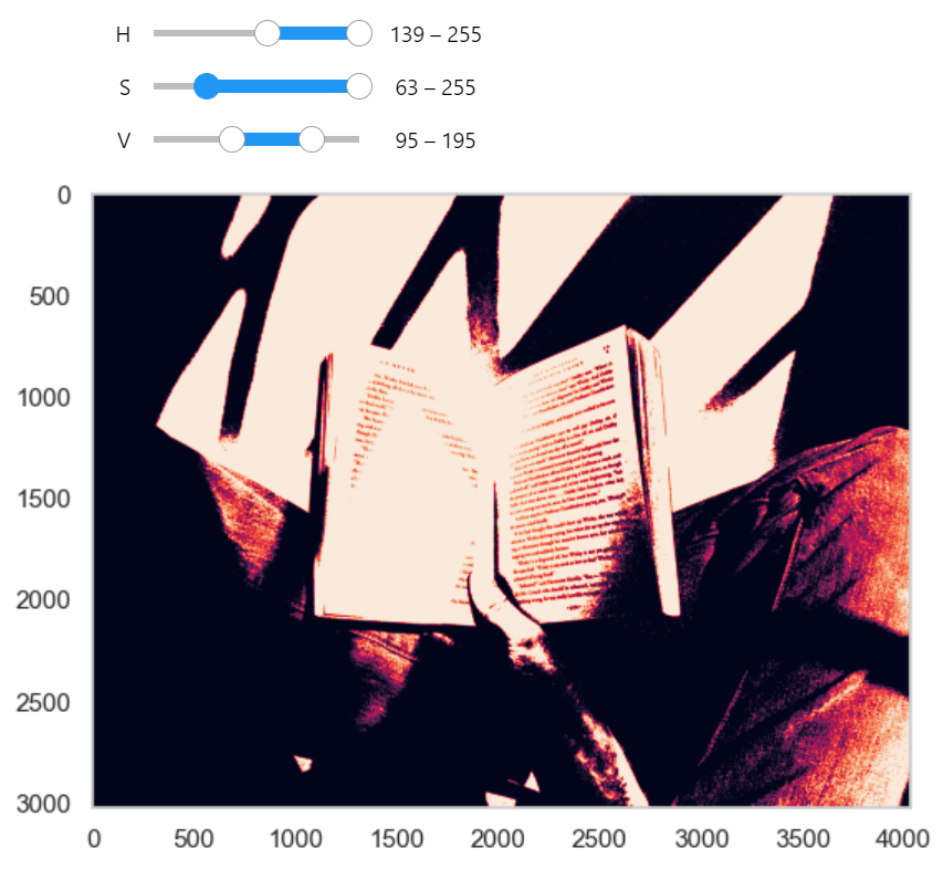
画像ヒストグラム確認
plt.hist(img_gray.ravel(),256,[0,256]); plt.show()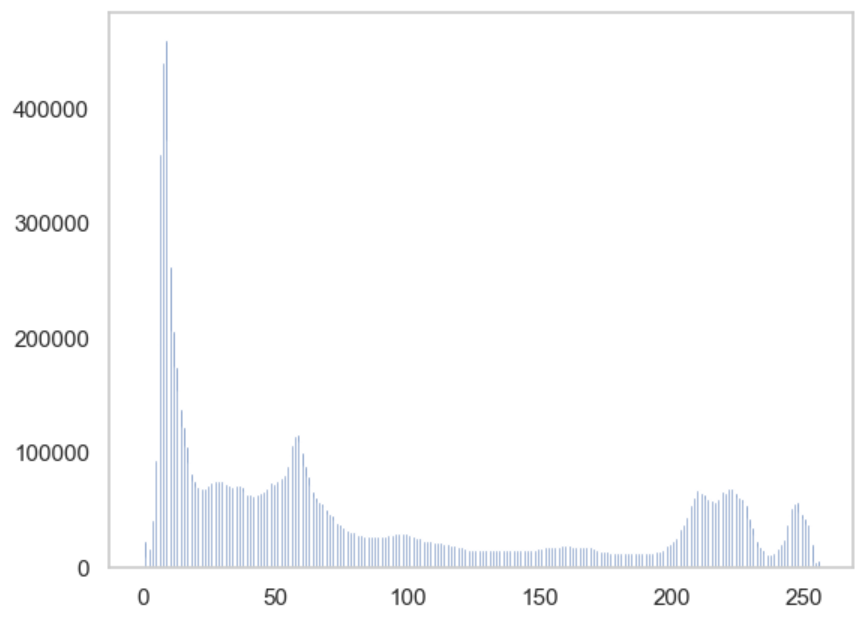
color = ('b','g','r')
label = ('b','g','r')
for i,col in enumerate(color):
    histr = cv2.calcHist([img_color],[i],None,[256],[0,256])
    plt.plot(histr,color = col, label=label[i])
    plt.xlim([0,256])
plt.legend()
plt.show()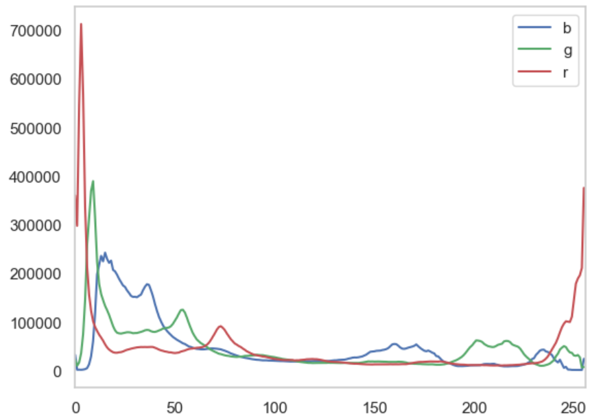
前処理 ノイズ除去
gauss = cv2.GaussianBlur(img_color,(15,15),3) # ガウシアンフィルタ
median = cv2.medianBlur(img_color,25) # 中央値フィルタ
bilate =  cv2.bilateralFilter(img_color,9,75,75) # バイラテラルフィルタ エッジが残りやすい
中央値フィルタの例
二値化
# 通常
_,img_gray_simple_thresh = cv2.threshold(img_gray,thresh=200,maxval=255,type=cv2.THRESH_BINARY)
plt.imshow(img_gray_simple_thresh,cmap='gray')
plt.show()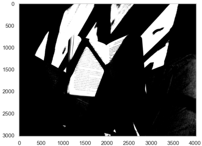
# 大津
_,img_gray_otsu_thresh = cv2.threshold(img_gray,thresh=0,maxval=255,type=cv2.THRESH_BINARY+cv2.THRESH_OTSU)
plt.imshow(img_gray_otsu_thresh,cmap='gray')
plt.show()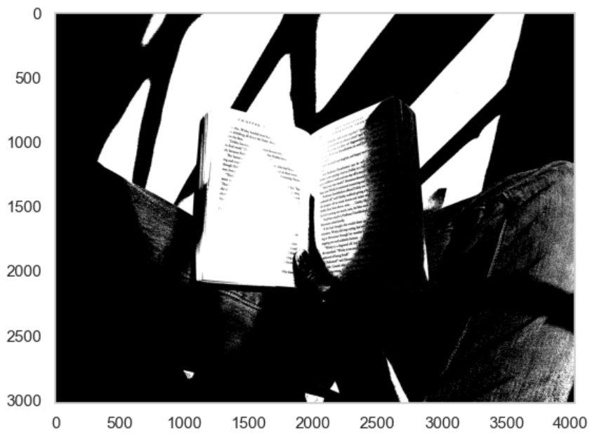
# 適応的二値化:平均
img_gray_adp_mean_thresh = cv2.adaptiveThreshold(img_gray,maxValue=255,adaptiveMethod=cv2.ADAPTIVE_THRESH_MEAN_C,thresholdType=cv2.THRESH_BINARY,blockSize=11,C=2)
plt.imshow(img_gray_adp_mean_thresh,cmap='gray')
plt.show()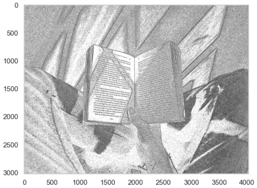
# 適応的二値化:ガウシアン
img_gray_adp_gauss_thresh = cv2.adaptiveThreshold(img_gray,maxValue=255,adaptiveMethod=cv2.ADAPTIVE_THRESH_GAUSSIAN_C,thresholdType=cv2.THRESH_BINARY,blockSize=11,C=2)
plt.imshow(img_gray_adp_gauss_thresh,cmap='gray')
plt.show()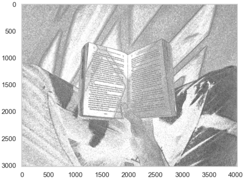
# 指定範囲で二値化
# 3チャネルの場合
lower = np.array([100, 0, 0]) # チャネルごとに下限値を指定
upper = np.array([200, 255, 255])  # チャネルごとに上限値を指定

img_range = cv2.inRange(img_hsv, lower, upper)
plt.imshow(img_range,cmap='gray')
plt.show()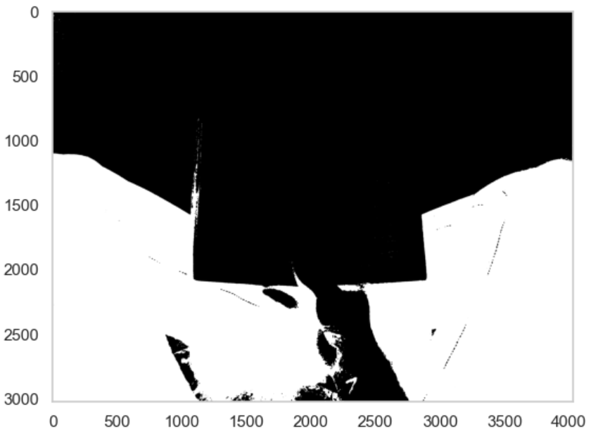
エッジ検出
edges = cv2.Canny(img_gray,100,200)
plt.imshow(edges,cmap = 'gray')
plt.show()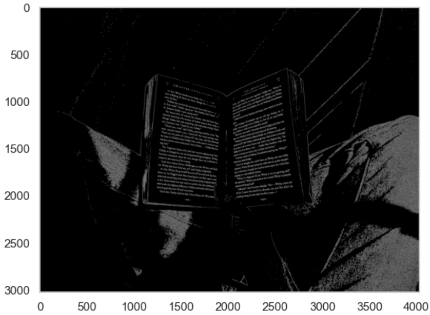
画像合成
lower = np.array([155, 0, 0]) # チャネルごとに下限値を指定
upper = np.array([165, 255, 255])  # チャネルごとに上限値を指定

img_range_strict = cv2.inRange(img_hsv, lower, upper)

replace_img_range = np.where(img_range == 255,127,img_range)
dst = cv2.add(img_range_strict,replace_img_range)
plt.imshow(dst,cmap='gray')
plt.colorbar()
plt.show()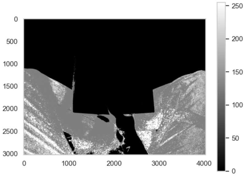


コメント